An introduction to the MXNet API — part 1
Update August 1st, 2017:
this series is now available in Japanese, Chinese and Korean.
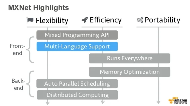
In this series, I will try to give you an overview of the MXnet Deep Learning library: we’ll look at its main features and its Python API (which I suspect will be the #1 choice). Later on, we’ll explore some of the MXNet tutorials and notebooks available online, and we’ll hopefully manage to understand every single line of code!
If you’d like learn more about the rationale and the architecture of MXNet, you should read this paper, named “MXNet: A Flexible and Efficient Machine Learning Library for Heterogeneous Distributed Systems”. We’ll cover most of the concepts presented in the paper, but hopefully in a more accessible way.
I’ll go as slow and explain as much as I need to. Expect minimal math and minimal jargon, but no (intentional) dumbing down. You won’t become an expert — I ain’t one anyway— but I hope you’ll learn enough to understand how you can add Deep Learning capabilities to your own applications.
Running MXNet locally
First things first: let’s install MXNet. You’ll find the official instructions here, but here are some additional tips.
One of the cool features of MXNet is that it can run identically on CPU and GPU (we’ll see later how to pick one or the other for our computations). This means that even if your computer doesn’t have an Nvidia GPU (just like my MacBook), you can still write and run MXNet code which you’ll use later on GPU-enabled systems.
If your computer has such a GPU, that’s great but you need to install the CUDA and cuDNN toolkits, which tends to turn into a nightmare more often than not. At the slightest incompatibility between the MXNet binary and the Nvidia tools, your setup will be broken and you won’t be able to work.
For this reason, I would strongly advise you to use the Docker images provided on the MXNet website: one for CPU environments, one for GPU environments (which requires nvidia-docker). These images come pre-installed with everything you need and allow you to get started in minutes.
sudo -H pip install mxnet  --upgrade
python
>>> import mxnet as mx
>>> mx.__version__
'0.9.3a3'
For what it’s worth, the Docker images also seem to be more up to date than the Python package available through ‘pip’.
docker run -it  mxnet/python
root@88a5fe9c8def:/# python
>>> import mxnet as mx
>>> mx.__version__
'0.9.5'
Running MXNet on AWS
AWS provides you with the Deep Learning AMI, available both for Linux and Ubuntu. This AMI comes pre-installed with many Deep Learning frameworks (MXNet included), as well as all the Nvidia tools and more. No plumbing needed.
====================================================================
       __|  __|_  )
       _|  (     /   Deep Learning AMI for Amazon Linux
      ___|\___|___|
====================================================================
[ec2-user@ip-172-31-42-173 ~]$ nvidia-smi -L
GPU 0: GRID K520 (UUID: GPU-d470337d-b59b-ca2a-fe6d-718f0faf2153)
[ec2-user@ip-172-31-42-173 ~]$ python
>>> import mxnet as mx
>>> mx.__version__
'0.9.3'
You can run this AMI either on a regular instance or on a GPU instance. If your computer doesn’t have an Nvidia GPU, this might come in handy later when we start training networks: your most inexpensive option will be to use a g2.2xlarge instance at $0.65 per hour.
For now, a good old-fashioned CPU is all we need! Let’s get started.
Why NDArrays are important
The first part of the MXNet API we’re going to look at in the NDArray API. An NDArray is an n-dimensional array, containing items of identical type and size (32-bit floats, 32-bit integers, etc).
Why are these arrays important? As explained in a previous article, training and running neural networks involve a lot of math operations. Multi-dimensional arrays is how we’ll store our data.
Input data, neuron weights and output data are stored in vectors and matrices, so it’s quite natural to have this kind of construct available.
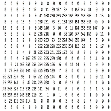
Let’s take a simple example: categorizing images. The image below represents an handwritten ‘8’, 18x18 pixels.

This image represents the same image as an 18x18 matrix, with each cell holding the greyscale value for the corresponding pixel: ‘0’ for white, ‘255’ for black and values in between for 254 shades of grey. This matrix representation is what we’ll run through a neural network to train it in categorizing digits from 0 to 9.
Now imagine that we use colour images instead of greyscale images. Each image would now be described using 3 matrices, one for each colour, so our input data is now a little more complicated.
Let’s go one step further. Imagine we’re doing real time image recognition for autonomous driving: in order to make decisions on quality up-to-date data, we’re using 1000 x 1000-pixel RGB images at 30 frames per second. Every second, we’ll have to handle 90 1000 x 1000 matrices (30 frames x 3 colours). If each pixel is represented as a 32-bit value, that’s 90 x 1000 x 1000 x 4 bytes, more or less 343 Megabytes. If you have multiple cameras, things add up pretty quick.
That’s a lot of data to pump through a neural network: for maximal performance (i.e. minimal latency), GPUs don’t process images one by one: instead, they process them in batches. If we use a batch size of 8, our neural network will process input data in chunks of 1000 x 1000 x 24, i.e. a 3-dimensional array holding 8 1000 x 1000 images in 3 colours.
Bottom line: you need to understand NDArrays :) They’re the bread and butter of neural networks, as they will be used to store pretty much all of our data.
The NDArray API
Now that we know why NDArrays are important, let’s look at how they work (yeah, code at last!). If you’ve worked with the numpy Python library, good news: NDArrays are extremely similar and you probably know most of the API, which is fully documented here.
Let’s start with the basics. No explanation needed, I suppose :)
>>> a = mx.nd.array([[1,2,3], [4,5,6]])
>>> a.size
6
>>> a.shape
(2L, 3L)
>>> a.dtype
<type 'numpy.float32'>
By default, an NDArray holds 32-bit floats, but we can customize that.
>>> import numpy as np
>>> b = mx.nd.array([[1,2,3], [2,3,4]], dtype=np.int32)
>>> b.dtype
Printing an NDArray is as easy as this.
>>> b.asnumpy()
array([[1, 2, 3],
       [2, 3, 4]], dtype=int32)
All the math operators you’d expect are available. Let’s try an element-wise matrix multiplication.
>>> a = mx.nd.array([[1,2,3], [4,5,6]])
>>> b = a*a
>>> b.asnumpy()
array([[  1.,   4.,   9.],
       [ 16.,  25.,  36.]], dtype=float32)
How about an proper matrix multiplication (aka ‘dot product’)?
>>> a = mx.nd.array([[1,2,3], [4,5,6]])
>>> a.shape
(2L, 3L)
>>> a.asnumpy()
array([[ 1.,  2.,  3.],
       [ 4.,  5.,  6.]], dtype=float32)
>>> b = a.T
>>> b.shape
(3L, 2L)
>>> b.asnumpy()
array([[ 1.,  4.],
       [ 2.,  5.],
       [ 3.,  6.]], dtype=float32)
>>> c = mx.nd.dot(a,b)
>>> c.shape
(2L, 2L)
>>> c.asnumpy()
array([[ 14.,  32.],
       [ 32.,  77.]], dtype=float32)
Let’s try something a little more complicated:
- initialize a 1000 x 1000 matrix with a uniform distribution, stored on GPU#0 (I’m using a g2 instance here).
- initialize another 1000 x 1000 matrix with a normal distribution (mean of 1 and standard deviation of 2), also on GPU#0.
>>> c = mx.nd.uniform(low=0, high=1, shape=(1000,1000), ctx="gpu(0)")
>>> d = mx.nd.normal(loc=1, scale=2, shape=(1000,1000), ctx="gpu(0)")
>>> e = mx.nd.dot(c,d)
Remember that MXNet can run identically on CPU and GPU. This is an example of this: just replace “gpu(0)” by “cpu(0)” in the previous example and now the dot product will run on the CPU.
You should now know enough to start playing with NDArrays. There are also higher level functions to build neural networks (FullyConnected, etc.) but we’ll study them when we start looking at actual networks.
That’s it for today. In the next post, we’ll look at the Symbol API, which allows us to define data flows, which is pretty much what neural networks are all about. Thanks for reading and stay tuned.