Training MXNet — part 1: MNIST
In a previous series, we discovered how we could use the MXNet library and pre-trained models for object detection. In this series, we’re going to focus on training models with a number of different data sets.
Let’s start with the famous MNIST data set.
Please note that is an updated and expanded version of this tutorial: I’m using the Module API (instead of the deprecated Model API) as well as the MNIST data iterator.
The MNIST data set
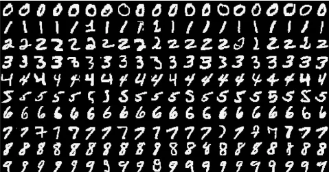
This data is a set of 28x28 greyscale images representing handwritten digits (0 to 9).
The training set has 60,000 samples and the test set has 10,000 examples. Let’s download them right away.
# Training set: images and labels
$ wget http://yann.lecun.com/exdb/mnist/train-images-idx3-ubyte.gz
$ wget http://yann.lecun.com/exdb/mnist/train-labels-idx1-ubyte.gz
# Validation set: images and labels
$ wget http://yann.lecun.com/exdb/mnist/t10k-images-idx3-ubyte.gz
$ wget http://yann.lecun.com/exdb/mnist/t10k-labels-idx1-ubyte.gz
$ gzip -d *
How about we take a look inside these files? We’ll start with the labels. They are stored as a serialized numpy array holding 60,000 unsigned bytes.
The file starts with a big-endian packed structure, holding 2 integers: magic number, number of labels.
>>> import struct
>>> import numpy as np
>>> import cv2
>>> labelfile = open("train-labels-idx1-ubyte")
>>> magic, num = struct.unpack(">II", labelfile.read(8))
>>> labelarray = np.fromstring(labelfile.read(), dtype=np.int8)
>>> print labelarray.shape
>>> print labelarray[0:10]
(60000,)
[5 0 4 1 9 2 1 3 1 4]
Let’s now extract some images. Again, they are stored as a serialized numpy array, which we will reshape to build 28x28 images. Each pixel is stored as an unsigned byte (0 for black, 255 for white).
The file starts with a big-endian packed structure, holding 4 integers: magic number, number of images, number of rows and number of columns.
>>> imagefile = open("train-images-idx3-ubyte")
>>> magic, num, rows, cols = struct.unpack(">IIII", imagefile.read(16))
>>> imagearray = np.fromstring(imagefile.read(), dtype=np.uint8)
>>> print imagearray.shape
(47040000,)
>>> imagearray = imagearray.reshape(num, rows, cols)
>>> print imagearray.shape
(60000, 28, 28)
Let’s save the first 10 images to disk.
>>> for i in range(0,10):
        img = imagearray[i]
        imgname = "img"+(str)(i)+".png"
        cv2.imwrite(imgname, img)
$ ls img?.png
img0.png img1.png img2.png img3.png img4.png img5.png img6.png img7.png img8.png img9.png
This is how they look.

Ok, now that we understand the data, let’s build a model.
Building a model
We’re going to use a simple multi-layer perceptron (similar to what we built here) : 784 → 128 → 64 → 10
- Input layer: an array of 784 pixel values (28x28).
- First layer: 128 neurons activated by the rectifier linear unit function.
- Second layer: 64 neurons activated by the same function.
- Output layer: 10 neurons (for our 10 categories), activated by the softmax function in order to transform the 10 outputs into 10 values between 0 and 1 that add up to 1. Each value represents the predicted probability for each category, the largest one pointing at the most likely category.
data = mx.sym.Variable('data')
data = mx.sym.Flatten(data=data)
fc1  = mx.sym.FullyConnected(data=data, name='fc1', num_hidden=128)
act1 = mx.sym.Activation(data=fc1, name='relu1', act_type="relu")
fc2  = mx.sym.FullyConnected(data=act1, name='fc2', num_hidden = 64)
act2 = mx.sym.Activation(data=fc2, name='relu2', act_type="relu")
fc3  = mx.sym.FullyConnected(data=act2, name='fc3', num_hidden=10)
mlp  = mx.sym.SoftmaxOutput(data=fc3, name='softmax')mod = mx.mod.Module(mlp)
Building a data iterator
MXNet conveniently provides a data iterator for the MNIST data set. Thanks to this, we don’t have to open the files, build NDArrays, etc. It also has default parameters for filenames and so on. Very cool!
train_iter = mx.io.MNISTIter(shuffle=True)
val_iter = mx.io.MNISTIter(image="./t10k-images-idx3-ubyte", label="./t10k-labels-idx1-ubyte")
We can now bind the data to our model. Default batch size is 128.
mod.bind(data_shapes=train_iter.provide_data, label_shapes=train_iter.provide_label)
We’re now ready for training.
Training the model
Let’s start with default settings for weight initialization and optimization (aka hyperparameters) and hope for the best. Here we go!
>>> import logging
>>> logging.basicConfig(level=logging.INFO)
>>> mod.fit(train_iter, num_epoch=10)
INFO:root:Epoch[0] Train-accuracy=0.111662
INFO:root:Epoch[0] Time cost=1.244
INFO:root:Epoch[1] Train-accuracy=0.112346
INFO:root:Epoch[1] Time cost=1.376
INFO:root:Epoch[2] Train-accuracy=0.112346
INFO:root:Epoch[2] Time cost=1.254
INFO:root:Epoch[3] Train-accuracy=0.112346
INFO:root:Epoch[3] Time cost=1.296
INFO:root:Epoch[4] Train-accuracy=0.112346
INFO:root:Epoch[4] Time cost=1.234
INFO:root:Epoch[5] Train-accuracy=0.112346
INFO:root:Epoch[5] Time cost=1.283
INFO:root:Epoch[6] Train-accuracy=0.112346
INFO:root:Epoch[6] Time cost=1.440
INFO:root:Epoch[7] Train-accuracy=0.112346
INFO:root:Epoch[7] Time cost=1.237
INFO:root:Epoch[8] Train-accuracy=0.112346
INFO:root:Epoch[8] Time cost=1.235
INFO:root:Epoch[9] Train-accuracy=0.112346
INFO:root:Epoch[9] Time cost=1.307
Hmm, things are not going well. It looks like the network is not learning. Actually, it is learning, but real slow: the default learning rate is 0.01, which is too low. Let’s use a more reasonable value such as 0.1.
>>> mod.init_params()
>>> mod.init_optimizer(optimizer_params=(('learning_rate', 0.1), ))
>>> mod.fit(train_iter, num_epoch=10)
INFO:root:Epoch[0] Train-accuracy=0.111846
INFO:root:Epoch[0] Time cost=1.288
INFO:root:Epoch[1] Train-accuracy=0.427150
INFO:root:Epoch[1] Time cost=1.308
INFO:root:Epoch[2] Train-accuracy=0.842682
INFO:root:Epoch[2] Time cost=1.271
INFO:root:Epoch[3] Train-accuracy=0.900875
INFO:root:Epoch[3] Time cost=1.282
INFO:root:Epoch[4] Train-accuracy=0.928736
INFO:root:Epoch[4] Time cost=1.288
INFO:root:Epoch[5] Train-accuracy=0.944478
INFO:root:Epoch[5] Time cost=1.296
INFO:root:Epoch[6] Train-accuracy=0.953993
INFO:root:Epoch[6] Time cost=1.287
INFO:root:Epoch[7] Train-accuracy=0.960453
INFO:root:Epoch[7] Time cost=1.294
INFO:root:Epoch[8] Train-accuracy=0.965478
INFO:root:Epoch[8] Time cost=1.297
INFO:root:Epoch[9] Train-accuracy=0.969267
INFO:root:Epoch[9] Time cost=1.291
That’s more like it. We get to 96.93% accuracy after 10 epochs. What about validation accuracy? Let’s create a metric and score our validation data set.
>> metric = mx.metric.Accuracy()
>> mod.score(val_iter, metric)
>> print metric.get()
('accuracy', 0.9654447115384616)
Pretty good accuracy at 96.5%.
Still, the first few training epochs are not great: this is caused by default weight initialization. Let’s use something smarter, like the Xavier technique.
>>> mod.init_params(initializer=mx.init.Xavier(magnitude=2.))
>>> mod.init_optimizer(optimizer_params=(('learning_rate', 0.1), ))
>>> mod.fit(train_iter, num_epoch=10)
INFO:root:Epoch[0] Train-accuracy=0.860994
INFO:root:Epoch[0] Time cost=1.338
INFO:root:Epoch[1] Train-accuracy=0.935797
INFO:root:Epoch[1] Time cost=1.325
INFO:root:Epoch[2] Train-accuracy=0.951840
INFO:root:Epoch[2] Time cost=1.273
INFO:root:Epoch[3] Train-accuracy=0.961438
INFO:root:Epoch[3] Time cost=1.264
INFO:root:Epoch[4] Train-accuracy=0.968066
INFO:root:Epoch[4] Time cost=1.250
INFO:root:Epoch[5] Train-accuracy=0.973174
INFO:root:Epoch[5] Time cost=1.299
INFO:root:Epoch[6] Train-accuracy=0.976846
INFO:root:Epoch[6] Time cost=1.374
INFO:root:Epoch[7] Train-accuracy=0.979601
INFO:root:Epoch[7] Time cost=1.407
INFO:root:Epoch[8] Train-accuracy=0.982121
INFO:root:Epoch[8] Time cost=1.336
INFO:root:Epoch[9] Train-accuracy=0.983958
INFO:root:Epoch[9] Time cost=1.343
>> metric = mx.metric.Accuracy()
>> mod.score(val_iter, metric)
>> print metric.get()
('accuracy', 0.9744591346153846)
That’s much better: we get to 86% accuracy after only one epoch. We gain almost 1.5% training accuracy and 1% validation accuracy.
Can we get better results? Well, we could always try to train the model longer. Let’s try 50 epochs.
...
INFO:root:Epoch[39] Train-accuracy=0.999950
INFO:root:Epoch[39] Time cost=1.284
INFO:root:Epoch[40] Train-accuracy=0.999967
INFO:root:Epoch[40] Time cost=1.301
INFO:root:Epoch[41] Train-accuracy=0.999967
INFO:root:Epoch[41] Time cost=1.811
INFO:root:Epoch[42] Train-accuracy=1.000000
INFO:root:Epoch[42] Time cost=1.412
INFO:root:Epoch[43] Train-accuracy=1.000000
INFO:root:Epoch[43] Time cost=1.275
INFO:root:Epoch[44] Train-accuracy=1.000000
INFO:root:Epoch[44] Time cost=1.200
...
('accuracy', 0.9785657051282052)
As you can see, we hit 100% training accuracy after 42 epochs and there’s no point in going any further. In the process, we only manage to improve validation accuracy by 0.4%.
Is this the best we can do? We could try other optimizers, but unless you really know what you’re doing, it’s probably safer to stick to SGD.
Maybe we simply need a bigger boat?
Using a deeper network
Let’s try this network and see what happens :
784 → 256 → 128 → 64 → 10
data = mx.sym.Variable('data')
data = mx.sym.Flatten(data=data)
fc1 = mx.sym.FullyConnected(data=data, name='fc1', num_hidden=256)
act1 = mx.sym.Activation(data=fc1, name='relu1', act_type="relu")
fc2  = mx.sym.FullyConnected(data=act1, name='fc2', num_hidden = 128)
act2 = mx.sym.Activation(data=fc2, name='relu2', act_type="relu")
fc3  = mx.sym.FullyConnected(data=act2, name='fc3', num_hidden = 64)
act3 = mx.sym.Activation(data=fc3, name='relu3', act_type="relu")
fc4  = mx.sym.FullyConnected(data=act3, name='fc4', num_hidden=10)
mlp  = mx.sym.SoftmaxOutput(data=fc4, name='softmax')
mod = mx.mod.Module(mlp)
mod.bind(data_shapes=train_iter.provide_data, label_shapes=train_iter.provide_label)
mod.init_params(initializer=mx.init.Xavier(magnitude=2.))
mod.init_optimizer(optimizer_params=(('learning_rate', 0.1), ))
mod.fit(train_iter, num_epoch=50)
We hit 100% training accuracy after 25 epochs and get to 97.99% validation accuracy, a modest 0.14% increase compared to the previous model. Clearly, a deeper multi-layer perceptron is not the way to go.
We need a better boat, then.
Using a Convolutional Neural Network
We’ve seen that these networks work very well for image processing. Let’s try a well-known CNN — called LeNet — on this data set.
Here is the model definition, everything else is identical.
data = mx.symbol.Variable('data')

conv1 = mx.sym.Convolution(data=data, kernel=(5,5), num_filter=20)
tanh1 = mx.sym.Activation(data=conv1, act_type="tanh")
pool1 = mx.sym.Pooling(data=tanh1, pool_type="max", kernel=(2,2), stride=(2,2))

conv2 = mx.sym.Convolution(data=pool1, kernel=(5,5), num_filter=50)
tanh2 = mx.sym.Activation(data=conv2, act_type="tanh")
pool2 = mx.sym.Pooling(data=tanh2, pool_type="max", kernel=(2,2), stride=(2,2))

flatten = mx.sym.Flatten(data=pool2)
fc1 = mx.symbol.FullyConnected(data=flatten, num_hidden=500)
tanh3 = mx.sym.Activation(data=fc1, act_type="tanh")

fc2 = mx.sym.FullyConnected(data=tanh3, num_hidden=10)

lenet = mx.sym.SoftmaxOutput(data=fc2, name='softmax')
mod.bind(data_shapes=train_iter.provide_data, label_shapes=train_iter.provide_label)
mod.init_params(initializer=mx.init.Xavier(magnitude=2.))
mod.init_optimizer(optimizer_params=(('learning_rate', 0.1), ))
mod.fit(train_iter, num_epoch=10)
Let’s train again.
INFO:root:Epoch[0] Train-accuracy=0.906634
INFO:root:Epoch[0] Time cost=46.034
INFO:root:Epoch[1] Train-accuracy=0.971989
INFO:root:Epoch[1] Time cost=47.089
This is painfully slow. About 45 seconds per epoch, about 30 times slower than the multilayer perceptron. Now would be a good time to try these fancy GPUs, don’t you think?
Training on a single GPU
By chance, I’ve running this on a g2.8xlarge instance. It has 4 NVidia GPUs ready to crunch data :)
[ec2-user]$ nvidia-smi -L
GPU 0: GRID K520 (UUID: GPU-5134e206-9b30-e1a8-a949-3d9e637a6465)
GPU 1: GRID K520 (UUID: GPU-221cb85e-2d26-b615-b674-ad596a8c12ee)
GPU 2: GRID K520 (UUID: GPU-ec4584ae-08e9-036f-d94a-ab60c52cf6fd)
GPU 3: GRID K520 (UUID: GPU-9bd3fe35-ac18-5d1a-4fb1-d819c9265ec2)
All it takes to switch from CPU to GPU is this. Amazing!
#mod = mx.mod.Module(lenet)
mod = mx.mod.Module(lenet, context=mx.gpu(0))
Here we go again.
INFO:root:Epoch[0] Train-accuracy=0.906651
INFO:root:Epoch[0] Time cost=3.452
INFO:root:Epoch[1] Train-accuracy=0.972022
INFO:root:Epoch[1] Time cost=3.455
INFO:root:Epoch[2] Train-accuracy=0.980786
INFO:root:Epoch[2] Time cost=3.450
INFO:root:Epoch[3] Train-accuracy=0.985210
INFO:root:Epoch[3] Time cost=3.454
INFO:root:Epoch[4] Train-accuracy=0.987931
INFO:root:Epoch[4] Time cost=3.454
INFO:root:Epoch[5] Train-accuracy=0.989633
INFO:root:Epoch[5] Time cost=3.453
INFO:root:Epoch[6] Train-accuracy=0.991036
INFO:root:Epoch[6] Time cost=3.449
INFO:root:Epoch[7] Train-accuracy=0.992238
INFO:root:Epoch[7] Time cost=3.451
INFO:root:Epoch[8] Train-accuracy=0.993323
INFO:root:Epoch[8] Time cost=3.453
INFO:root:Epoch[9] Train-accuracy=0.994191
INFO:root:Epoch[9] Time cost=3.452
('accuracy', 0.9903846153846154)
Nice! Training time has been massively reduced. Accuracy is now 99+% thanks to the more sophisticated model.
Did I mention that there are four GPUs in this box? How about using more than one?
Training on multiple GPUs
Once again, this is pretty simple to set up.
#mod = mx.mod.Module(lenet, context=mx.gpu(0))
mod = mx.mod.Module(lenet, context=(mx.gpu(0), mx.gpu(1)))
INFO:root:Epoch[0] Train-accuracy=0.906701
INFO:root:Epoch[0] Time cost=2.592
INFO:root:Epoch[1] Train-accuracy=0.972055
INFO:root:Epoch[1] Time cost=2.329
INFO:root:Epoch[2] Train-accuracy=0.980819
INFO:root:Epoch[2] Time cost=2.302
INFO:root:Epoch[3] Train-accuracy=0.985193
INFO:root:Epoch[3] Time cost=2.302
INFO:root:Epoch[4] Train-accuracy=0.987981
INFO:root:Epoch[4] Time cost=2.297
INFO:root:Epoch[5] Train-accuracy=0.989583
INFO:root:Epoch[5] Time cost=2.302
INFO:root:Epoch[6] Train-accuracy=0.991119
INFO:root:Epoch[6] Time cost=2.305
INFO:root:Epoch[7] Train-accuracy=0.992238
INFO:root:Epoch[7] Time cost=2.303
INFO:root:Epoch[8] Train-accuracy=0.993273
INFO:root:Epoch[8] Time cost=2.297
INFO:root:Epoch[9] Train-accuracy=0.994174
INFO:root:Epoch[9] Time cost=2.307
We saved 50% of training time. Let’s go for three GPUs.
#mod = mx.mod.Module(lenet, context=(mx.gpu(0), mx.gpu(1)))
mod = mx.mod.Module(lenet, context=(mx.gpu(0), mx.gpu(1), mx.gpu(2)))
INFO:root:Epoch[0] Train-accuracy=0.906667
INFO:root:Epoch[0] Time cost=1.938
INFO:root:Epoch[1] Train-accuracy=0.972055
INFO:root:Epoch[1] Time cost=1.924
INFO:root:Epoch[2] Train-accuracy=0.980836
INFO:root:Epoch[2] Time cost=1.916
INFO:root:Epoch[3] Train-accuracy=0.985193
INFO:root:Epoch[3] Time cost=1.903
INFO:root:Epoch[4] Train-accuracy=0.987997
INFO:root:Epoch[4] Time cost=1.910
INFO:root:Epoch[5] Train-accuracy=0.989600
INFO:root:Epoch[5] Time cost=1.910
INFO:root:Epoch[6] Train-accuracy=0.991052
INFO:root:Epoch[6] Time cost=1.912
INFO:root:Epoch[7] Train-accuracy=0.992288
INFO:root:Epoch[7] Time cost=1.921
INFO:root:Epoch[8] Train-accuracy=0.993339
INFO:root:Epoch[8] Time cost=1.934
INFO:root:Epoch[9] Train-accuracy=0.994157
INFO:root:Epoch[9] Time cost=1.937
('accuracy', 0.9904847756410257)
Another 20% saved. Training time is now only 50% more than what it was for the CPU-version of the multi-layer perceptron.
Adding a fourth GPU won’t help. Yes, I tried :) Anyway, we’re pretty happy with our model, so let’s save it for future use.
Saving our model
Saving a model just requires a file name and an epoch number.
mod.save_checkpoint("lenet", 10)This creates two files (which you should now be familiar with):
- the symbol file, containing the model definition (3.5KB)
- the parameter file, containing all our trained parameters (1.7MB)
$ ls lenet*
lenet-0010.params  lenet-symbol.json
Reusing our model
Just like we did in previous articles, we’re now able to load this pre-trained model.
lenet, arg_params, aux_params = mx.model.load_checkpoint("lenet", 10)
mod = mx.mod.Module(lenet)
mod.bind(for_training=False, data_shapes=[('data', (1,1,28,28))])
mod.set_params(arg_params, aux_params)
Here are the ugly digits I created with Paintbrush :)

I saved them as a 28x28 images, which I can now load as numpy arrays. I need to normalize pixels values and add two dimensions to reshape the array from (28, 28) to (1, 1, 28, 28) : batch size of one, one channel (greyscale), 28 x 28 pixels.
def loadImage(filename):
        img = cv2.imread(filename, cv2.IMREAD_GRAYSCALE)
        img = img / 255
        print img
        img = np.expand_dims(img, axis=0)
        img = np.expand_dims(img, axis=0)
        return mx.nd.array(img)
We’ll predict image by image. To avoid building a data iterator, I’ll use the same trick we’ve seen before (using a namedtuple to provide a data attribute).
def predict(model, filename):
        array = loadImage(filename)
        Batch = namedtuple('Batch', ['data'])
        mod.forward(Batch([array]))
        pred = mod.get_outputs()[0].asnumpy()
        return pred
Now we’re ready. Let check these digits!
np.set_printoptions(precision=3, suppress=True)
mod = loadModel()
print predict(mod, "./0.png")
print predict(mod, "./1.png")
print predict(mod, "./2.png")
print predict(mod, "./3.png")
print predict(mod, "./4.png")
print predict(mod, "./5.png")
print predict(mod, "./6.png")
print predict(mod, "./7.png")
print predict(mod, "./8.png")
print predict(mod, "./9.png")
And here are the results.
[[ 1.  0.  0.  0.  0.  0.  0.  0.  0.  0.]]
[[ 0.  1.  0.  0.  0.  0.  0.  0.  0.  0.]]
[[ 0.  0.  1.  0.  0.  0.  0.  0.  0.  0.]]
[[ 0.  0.  0.  1.  0.  0.  0.  0.  0.  0.]]
[[ 0.  0.  0.  0.  1.  0.  0.  0.  0.  0.]]
[[ 0.  0.  0.  0.  0.  1.  0.  0.  0.  0.]]
[[ 0.  0.  0.  0.  0.  0.  1.  0.  0.  0.]]
[[ 0.  0.  0.  0.  0.  0.  0.  1.  0.  0.]]
[[ 0.  0.  0.  0.  0.  0.  0.  0.  1.  0.]]
[[ 0.  0.  0.  0.001  0.009  0.  0. 0.002  0. 0.988]]
Wow. Hardly any doubt on the first 9 digits (probabilities are 99.99+%). Only my ugly 9 scores lower :)
Well, who thought that we’d have so much fun and that we’d cover so much ground using the MNIST dataset? Code and images are available on Github. Hopefully, this will get you started on building and training networks on your own data.
That’s it for today. Stay tuned for part 2 where we’ll look at another data set!