Training MXNet — part 2: CIFAR-10
In part 1, we used the famous LeNet Convolutional Neural Network to reach 99+% validation accuracy in just 10 epochs. We also saw how to use multiple GPUs to speed up training.
In this article, we’re going to tackle a more difficult data set: CIFAR-10. In the process, we’re going to learn a few new tricks. Read on :)
The CIFAR-10 data set
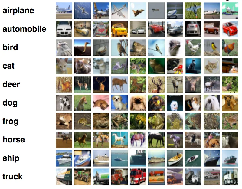
The CIFAR-10 dataset consists of 60,000 32 x 32 colour images. They are divided in 10 classes containing 6,000 images each. There are 50,000 training images and 10,000 test images. Categories are stored in a separate metadata file.
Let’s download the data set.
$ wget https://www.cs.toronto.edu/~kriz/cifar-10-python.tar.gz
$ tar xfz cifar-10-python.tar.gz
$ ls cifar-10-batches-py/
batches.meta  data_batch_1  data_batch_2  data_batch_3  data_batch_4  data_batch_5  readme.html  test_batch
Each file contains 10,000 pickled images, which we need to turn into an array shaped (10000, 3, 32, 32). The ‘3’ dimension comes for the three RGB channels, remember? :)
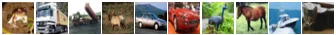
Let’s open the first file, save its first 10 images to disk and print their category. Nothing really complicated here, except some OpenCV tricks (see comments in the code below).
Here’s the output.
(10000, 3, 32, 32)
10000
['frog', 'truck', 'truck', 'deer', 'automobile', 'automobile', 'bird', 'horse', 'ship', 'cat']
Now let’s load the data set.
Loading CIFAR-10 in NDArrays
Just like we did for the the MNIST data, the CIFAR-10 images and labels could be loaded in NDArrays and then fed to an iterator. This is how we would to it.
Here’s the output.
(50000L, 3L, 32L, 32L)
(50000L,)
(10000L, 3L, 32L, 32L)
(10000L,)
The next logical step would be to bind these arrays to a Module and start training (just like we did for the MNIST data set). However, I’d like to show you another way to load image data: the RecordIO file.
Loading CIFAR-10 with RecordIO files
Being able to load data efficiently is a very important part of MXNet: you’ll find architecture details here. In a nutshell, RecordIO files allow large data sets to be packed and split in multiple files, which can then be loaded and processed in parallel by multiple servers for distributed training.
We won’t cover how to build these files today. Let’s use pre-existing files hosted on the MXNet website.
$ wget http://data.mxnet.io/data/cifar10/cifar10_val.rec
$ wget http://data.mxnet.io/data/cifar10/cifar10_train.rec
The first file contains 50,000 samples, which we’ll use for training. The second one contains 10,000 samples, which we’ll use for validation. Image resolution has been set to 28x28.
Loading these files and building an iterator is extremely simple. We just have to be careful to :
- match data_name and label_name with the names of the input and output layers.
- shuffle samples in the training set in case they’ve been stored in some kind of sequence.
Data is ready for training. We’ve learned from previous examples that Convolutional Neural Networks are a good fit for object detection, so that’s where we should look.
Training vs. fine-tuning
In previous examples, we picked models from the model zoo and retrained them from scratch on our data set. We’re going to do that again with the ResNext-101 model, but we’re going to try something different in parallel: fine-tuning the model.
Fine-tuning means that we’re going to keep all layers and pre-trained weights unchanged, except for the last layer: it will be removed and replaced by a new layer having the number of outputs of the new data set. Then, we will train the output layer on the new data set.
Since our model has been pre-trained on the large ImageNet data set, the rationale for fine-tuning is to benefit from the very large number of patterns that the model has learned while training on ImageNet. Although image sizes are quite different, it’s reasonable to expect that they will also apply to CIFAR-10.
Training on ResNext-101
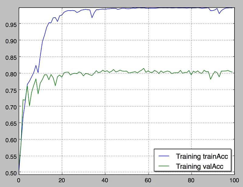
Let’s first start by training the model from scratch. We’ve done this a few times before, so no difficulty here.
This is the result after 100 epochs.
Fine-tuning on ResNext-101
Replacing layers sounds complicated, doesn’t it? Fortunately, the MXNet sources provide Python code to do this. It’s located in example/image-classification/fine-tune.py. Basically, it’s going to download the pre-trained model, remove its output layer, add a new one and start training.
This is how to use it:
$ python fine-tune.py
--pretrained-model resnext-101 --load-epoch 0000
--gpus 0,1,2,3 --batch-size 128
--data-train cifar10_train.rec --data-val cifar10_val.rec
--num-examples 50000 --num-classes 10 --image-shape 3,28,28
--num-epoch 300 --lr 0.05
This is going to download resnext-101–0000.params and resnext-101-symbol.json from the model zoo. Most of the parameters should be familiar. Here’s the result after 100 epochs.
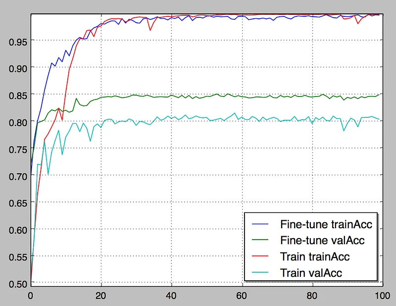
What do we see here?
Early on, fine-tuning delivers much higher training and validation accuracy. This makes sense, since the model has been pre-trained. So, if you have limited time and resources, fine-tuning is definitely an interesting way to get quick results on a new data set.
Over time, fine-tuning delivers about 5% additional validation accuracy than training from scratch. I’m guessing that the pre-trained model generalizes better on new data thanks to the large ImageNet data set.
Last but not least, validation accuracy stops improving after 50 epochs or so. Surely, we can do something to improve this?
Yes, of course. We’ll see how in part 3 :)