Generative Adversarial Networks on Apache MXNet, part 1

In several previous posts, I’ve shown you how to classify images using a variety of Convolution Neural Networks. Using a labeled training set and applying a supervised learning process, AI delivers fantastic results on this problem and on similar ones, such as object detection or object segmentation.

Impressive as it is, this form of intelligence only deals with understanding representations of our world as it is (text, images, etc). What about inventing new representations? Could AI be able to generate brand new images, convincing enough to fool the human eye? Well, yes.

In this post, we’ll start to explore how!

Generative Adversarial Networks

A breakthrough happened in 2014, with the publication of “Generative Adversarial Networks”, by Ian J. Goodfellow, Jean Pouget-Abadie, Mehdi Mirza, Bing Xu, David Warde-Farley, Sherjil Ozair, Aaron Courville and Yoshua Bengio.

In my crystal ball, I see Ian Goodfellow winning a Turing Award for this. It might take 30 years, but mark my words.

Relying on an unlabeled data set and an unsupervised learning process, GANs are able to generate new images (people, animals, landscapes, etc.) or even alter parts of an existing image (like adding a smile to a person’s face).

An intuitive explanation

The original Goodfellow article uses the art forger vs art expert analogy, which has been rehashed to death on countless blogs. I’ll let you read the original version and I’ll try to use a different analogy: cooking.

You’re the apprentice and I’m the chef (obviously!). Your goal would to cook a really nice Boeuf Bourguignon, but I wouldn’t give you any instructions. No list of ingredients, no recipe, nothing. My only request would be: “cook something with 20 ingredients”.

You’d go the pantry, pick 20 random ingredients, mix them together in a pot and show me the result. I’d look at it and of course the result would be nothing like what I expected

For each of the ingredients you selected, I’d give you a hint which would help you get a little bit closer to the actual recipe. For example, if you picked chicken, I could tell you: “Well, there is no chicken in this recipe but there is meat”. And if you used grape juice, I may say: “Hmm, the color is right but this is the wrong liquid” (red wine is required).

Resolved to improve, you’d go back to the pantry and try to make slightly better choices. The result would still be far off, but a little bit closer anyway. I’d give you more hints, you’d cook again and so on. After a number of iterations (and a massive waste of food), chances are you’d get very close to the actual recipe — assuming that I wouldn’t have lost my temper by then :D

A (slightly) more scientific explanation

Let’s replace the apprentice by the Generator and the chef by the Discriminator. Here is how GANs work.

1. The Generator model has no access to the data set. Using random data, it creates an image that is forwarded through the Detector model.
2. The Discriminator model learns how to recognise valid data samples (the ones included in the data) from invalid data samples (the ones computed by the Generator). The training process uses traditional techniques like gradient descent and back propagation.
3. The Generator model also learns, but in a different way. First, it treats its samples as valid (it’s trying to fool the Discriminator after all). Second, weights are updated using the gradients computed by the Discriminator.
4. Repeat!

This is the key to understanding GANs: by treating its samples as valid and by applying the Discriminator weight updates, the Generator progressively learns how to generate data samples that are closer and closer to the ones that the Discriminator considers as valid, i.e. the ones that are part of the data set.

Brilliant, brilliant idea (Turing award, I’m telling you).

Deep Convolutional GANs

GANs may be implemented using a number of different model architectures. Here, we will study a GAN based on Convolutional Neural Networks, as published in “Unsupervised Representation Learning with Deep Convolutional Generative Adversarial Networks”, by Alec Radford, Luke Metz and Soumith Chintala (2016).

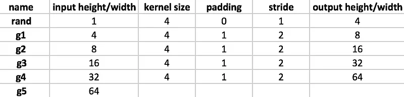
Let’s take a look at the Generator model. I’ve slightly updated the illustration included in the original article to reflect the exact code that we will use later on.

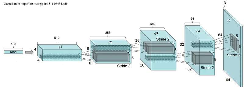
Don’t panic, it’s not as bad as you think. We start from a random vector of 100 values. Using 5 transposed convolution operations (more on this in a minute), this vector is turned into an RGB 64x64 image (hence the 3 channels).

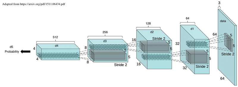
Now let’s look at the Discriminator. Wait, it’s almost identical (don’t forget to start from the left this time). Using 5 convolution operations, we turn an RGB 64x64 image into a probability: true for valid samples, false for invalid samples.

Still with me? Good. Now what about this convolution / transposed convolution thing?

A look at convolution

There are plenty of great tutorials out there. The best I’m aware of is part of the Theano documentation. Extremely detailed with beautiful animations. Read it and words like “kernel”, “padding” and “stride” will become crystal clear.

In a nutshell, convolution is typically used to reduce dimensions. This is why this operation is at the core of Convolutional (duh) Neural Networks: they start from a full image (say 224x224) and gradually shrink it through a series of convolutions which will only preserve the features that are meaningful for classification.

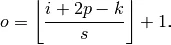
The formula to compute the size of the output image is actually quite simple.

We can apply it to the Discriminator network above and yes, it works. Woohoo.

A look at transposed convolution

Transposed convolution is the reverse process, i.e. it increases dimensions. Don’t call it “Deconvolution”, it seems to aggravate some people ;)

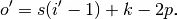
The formula to compute the size of the output image is as follows.

Applying it to the Generator network gives us the correct results too. Hopefully, this is starting to make sense and you now understand how it’s possible to generate a picture from a vector of random values :)

Coding the Discriminator network

Apache MXNet has a couple of nice examples implementing this network architecture in R and Python. I’ll use Python for the rest of the post, but I’m sure R users will follow along.

Here’s the code for the Discriminator network, based on the illustration above. You’ll find extra details in the research article, e.g. why they use the LeakyRelu activation function and so on.

Coding the Generator network

Here’s the code for the Generator network, based on the illustration above.

Preparing MNIST

OK, now let’s take care of the data set. As you probably know, the MNIST data set contains 28x28 black and white images. We need to:

• reshape them to 64x64 images,
• normalize pixel values between 0 and 1,
• add two extra channels (identical to the original image),
• set 10,000 samples aside to validate the Discriminator.

Nothing MXNet-specific here, just good old Python data manipulation.

During Discriminator training, this data set will be served by a standard NDArray iterator.

Preparing random data

We also need to provide random data to the Generator. We’ll do this with a custom iterator.

When getdata() is called, this iterator will return an NDArray shaped (batch size, random vector size, 1, 1). We’ll use a 100-element random vector, so through multiple transposed convolutions, the Generator will indeed build a picture from a (100, 1, 1) sample.

The training loop

Time to look at the training code. This time, we cannot use the Module.fit() API. We have to write a custom training loop taking into account the fact that we’re going to use the Discriminator gradients to update the Generator.

Here are the steps:

1. Generate a batch of random samples (line 4).
2. Forward the batch through the Generator and grab the resulting images (lines 6–7).
3. Label these images as fake, forward them through the Discriminator and run back propagation (lines 10–12) : this lets the Discriminator learn to detect fake images.
4. Save the Discriminator gradients but do not update the Discriminator weights at the moment (line 13).
5. Label the current MNIST batch of images as real images, forward them through the Discriminator and run back propagation (lines 16–19) : this lets the Discriminator learn to detect real images.
6. Add the “fake images” gradients to the “real images” gradients and update the Discriminator weights (lines 20–23).
7. Label the Generator images as real this time, forward them through the Discriminator again and run back propagation (lines 26–28).
8. Get the Discriminator gradients: they would normally help the Discriminator learn how real images look like. However, we’re applying them to the Generator network instead, effectively helping it to forge better fake images (lines 29–31).

Quite a mouthful! Congratulations if you got this far: you understood the core concepts of GANs.

Let’s run this thing

The MXNet sample includes code to visualize the images coming out of the Generator . The simplest way to view them is to copy the code in a Jupyter notebook and run it :)

After a few minutes (especially if you use a Volta-powered p3 instance), you should see something similar to this.

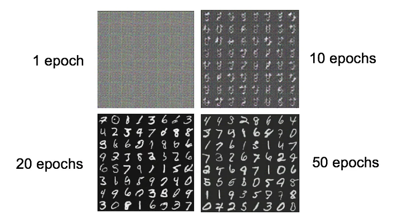
As you can see, random noise gradually turns into well-formed digits. It’s just math, but it’s still amazing…

In all chaos there is a cosmos, in all disorder a secret order— Carl Jung

So when do we stop training?

Common training metrics like accuracy mean nothing here. We have no way of knowing whether Generator images are getting better… except by looking at them.

An alternative would be to generate only fives (or any other digit), to run them through a proper MNIST classifier and to measure accuracy.

There is also ongoing research to use new metrics for GANs, such as the Wasserstein distance. Let’s keep this topic for another article :)

Thanks for reading. This is definitely a deeper dive than usual, but I hope you enjoyed it.

Only one song is worthy here. Generator vs Discriminator, may the best model win!